Bayesian Portfolio Optimization
Max Margenot
Lead - Data Science at Quantopian
This presentation is for informational purposes only and does not constitute an offer to sell, a solicitation to buy, or a recommendation for any security; nor does it constitute an offer to provide investment advisory or other services by Quantopian, Inc. ("Quantopian"). Nothing contained herein constitutes investment advice or offers any opinion with respect to the suitability of any security, and any views expressed herein should not be taken as advice to buy, sell, or hold any security or as an endorsement of any security or company. In preparing the information contained herein, Quantopian, Inc. has not taken into account the investment needs, objectives, and financial circumstances of any particular investor. Any views expressed and data illustrated herein were prepared based upon information, believed to be reliable, available to Quantopian, Inc. at the time of publication. Quantopian makes no guarantees as to their accuracy or completeness. All information is subject to change and may quickly become unreliable for various reasons, including changes in market conditions or economic circumstances.
Background
- Me
The Problem
In finance, a base unit of work is the creation of some sort of portfolio
This can be simple or complex
Risk
What is risk?
Something you don't want?
Something you do want?
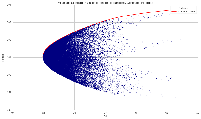
Modern Portfolio Theory
A framework for finding portfolios that maximize expected return while minimizing risk.
Portfolio Diversification
- Constant advice.
- Important at all levels of investment.
A Simple Example
mu = np.mean(returns, axis=1) - 1
sigma = np.std(returns, axis=1)

weights = np.array([1./N for asset in mu])
print('Asset Returns are: ', mu)
print('Asset Volatilities are: ', sigma)
print('Portfolio Return is: ', mu.dot(weights))
print('Portfolio Volatility is: ', np.sqrt((weights**2).dot(sigma**2)))
Generalization
$$ P = \sum_{i=1}^N \omega_i S_i $$
$$ E[\mu_P] = \sum_{i=1}^N \omega_i \mu_i $$
$$ VAR[P] = \sigma_p^2 = \sum_{i=1}^N \omega_i^2 \sigma_i^2 + \sum_{i=1}^N \sum_{j=1, j\neq i}^N \omega_i\omega_j \sigma_i\sigma_j \rho_{ij}$$
Portfolio Optimization
Given a potentially massive universe of securities available to trade, what is the best way to combine the assets you want?
Is there a "correct" way to determine $\{\omega_i\}_{i=1}^N$?
We can express this as a conventional optimization problem, with objective and constraints.
Markowitz Portfolio Optimization
Given a set of assets, $\{S_i\}_{i=1}^N$, with expected returns $\{R_i\}_{i=1}^N$ and covariance matrix $\Sigma$,
\begin{equation*} \begin{aligned} & \underset{\omega} {\text{minimize}} & & \omega^\top\Sigma\omega - R^\top\omega \\ & \text{subject to} & & \sum_{i=1}^N \omega_i = 1 \end{aligned} \end{equation*}
- We're still riffing on this.
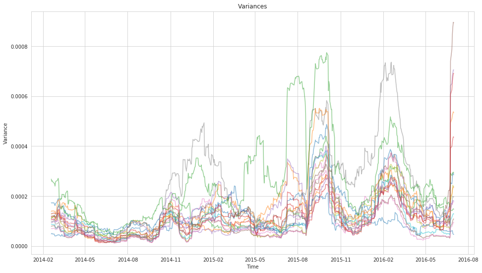
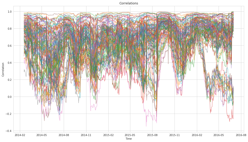
Why is this Hard?
- Traditional covariance is unstable.
- Too many observations are necessary to make it stable.
- Correlations change over time.
- There's a Wikipedia article about this, so it must be: https://en.wikipedia.org/wiki/Estimation_of_covariance_matrices.
But Let's Take a Step Back
Uncertainty gives us strength.
In finance, this gives us even more confidence.
Bayesian Statistics
Bayesian statistics is a statistical framework for quantifying uncertainty in the form of probability distributions.
$$ P(\theta\ |\ \mathbf{X}) = \frac{P(\mathbf{X}\ |\ \theta)\ P(\theta)}{P(\mathbf{X})} \propto P(\mathbf{X}\ |\ \theta)\ P(\theta) $$
- $P(\theta\ |\ \mathbf{X})$ is our posterior distribution.
- $P(\mathbf{X}\ |\ \theta)$ is the likelihood of the model.
- $P(\theta)$ is our prior distribution.
Prior Work
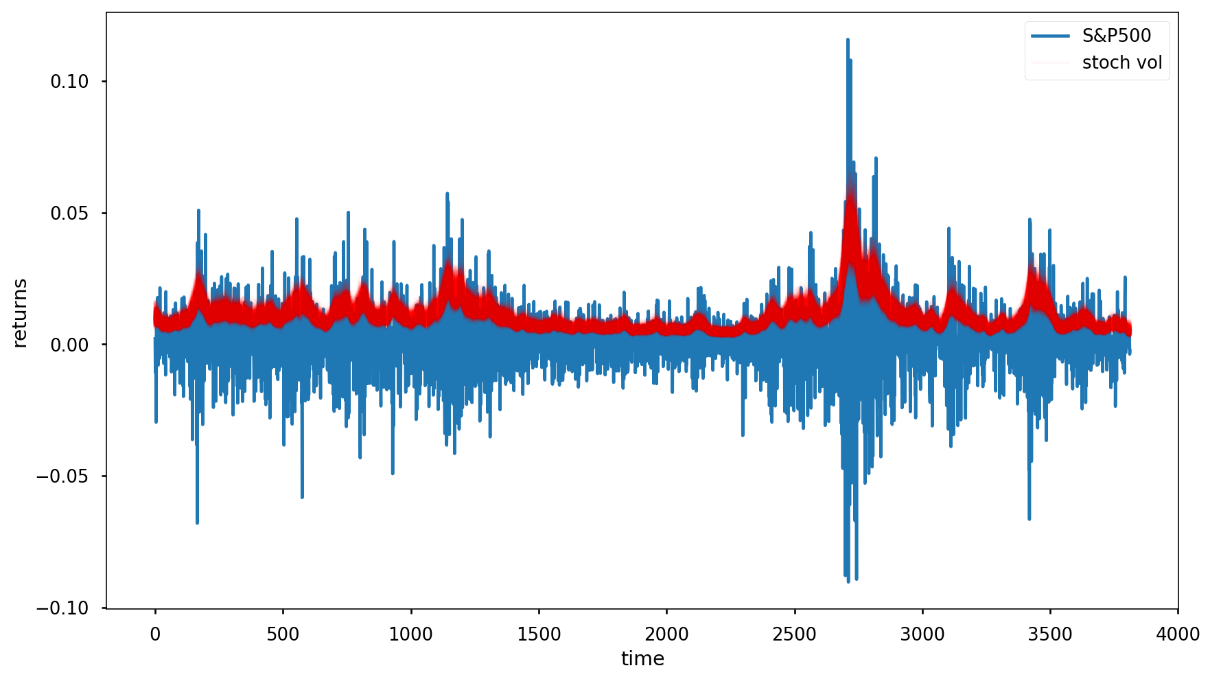
Probabilistic Programming
Probabilistic programming is a tool that helps us express this problem using code.
We set our priors and our likelihood and the sampler does the heavy lifting.
with pm.Model() as model:
    step_size = pm.Exponential('sigma', 50.)
    s = GaussianRandomWalk('s', sd=step_size,
                           shape=len(returns))

    nu = pm.Exponential('nu', .1)

    r = pm.StudentT('r', nu=nu,
                    lam=pm.math.exp(-2*s),
                    observed=returns)
def build_basic_rw_model(observations, subsample_rate=30):
    total_time, n_secs = observations.shape
    with pm.Model() as bayesian_cov:
        log_var = pm.GaussianRandomWalk(
            "log_var",
            mu=0,
            sd=.1,
            shape=(total_time//subsample_rate, n_secs),
        )
        var = tt.exp(log_var)

        lower_chol = pm.GaussianRandomWalk(
            "lower_chol",
            mu=0,
            sd=.1,
            shape=(total_time//subsample_rate, n_secs*(n_secs-1)//2)
        )
        cholesky = tt.as_tensor(
            [expand_diag_lower(n_secs, var[t,:], lower_chol[t,:])
                for t in range(total_time//subsample_rate)])

        covariance = pm.Deterministic(
            'covariance',
            tt.as_tensor([cholesky[t].dot(cholesky[t].T)
                          for t in range(total_time//subsample_rate)])
        )

        reshaped_returns = observations.values[
            :(subsample_rate*(total_time//subsample_rate))
        ].reshape(total_time//subsample_rate, subsample_rate, n_secs)
        time_segments, _, _ = reshaped_returns.shape

        for t in range(time_segments):
            pm.MvNormal(
                'likelihood_{0}'.format(t),
                mu=np.zeros(n_secs),
                chol=cholesky[t,:,:],
                observed=reshaped_returns[t]
            )
    return bayesian_cov
with model:
    trace = pm.sample(1000, tune=1000, njobs=2)
Probabilistic Programming
With this in mind, we set the following priors for our returns and covariance matrix:
\begin{eqnarray*} R &\sim& MvNormal(0, \Sigma) \\ L &\sim& \exp[GaussianRandomWalk(0, 0.1)]\\ \Sigma &=& LL^\top \end{eqnarray*}
where $\Sigma = LL^\top$ is the Cholesky decomposition of $\Sigma$.
Trading Universe
17 ETFs, examined in a previous post from the Quantopian Forums.
rets.head()
Trace
pm.traceplot(basic_trace);

Diagnostics
gr_stats = pm.diagnostics.gelman_rubin(basic_trace)
print("Average Gelman-Rubin Statistics:")
for variable, stats in gr_stats.items():
    print("{0}: {1}".format(variable, np.mean(stats)))
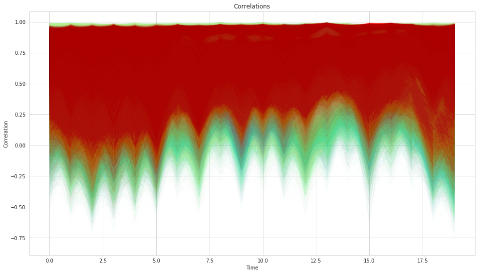
Posteriors
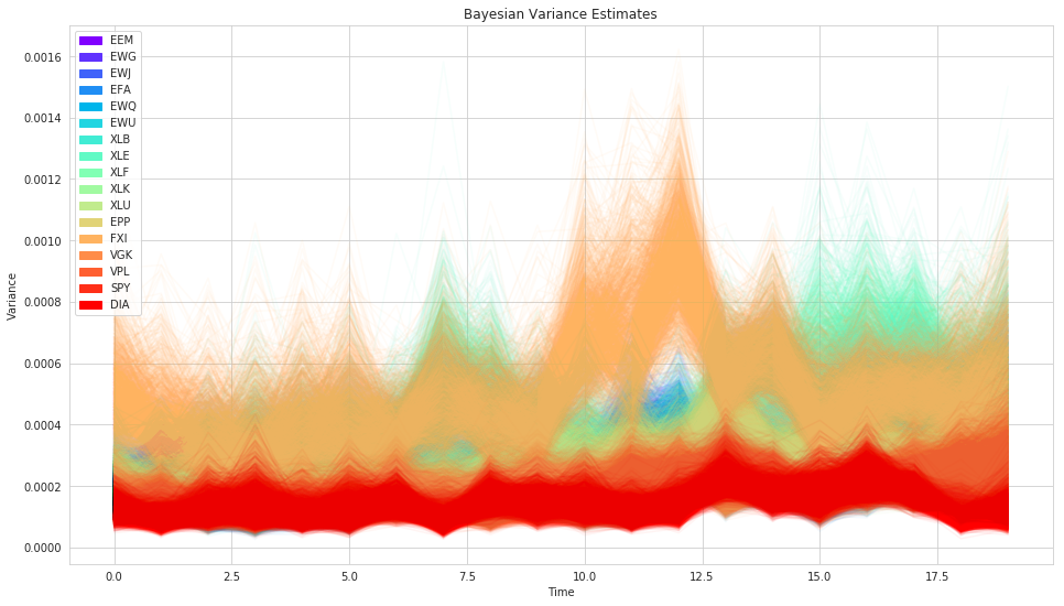
Posteriors
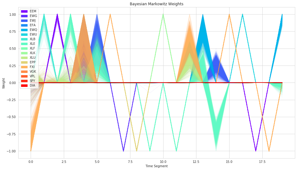
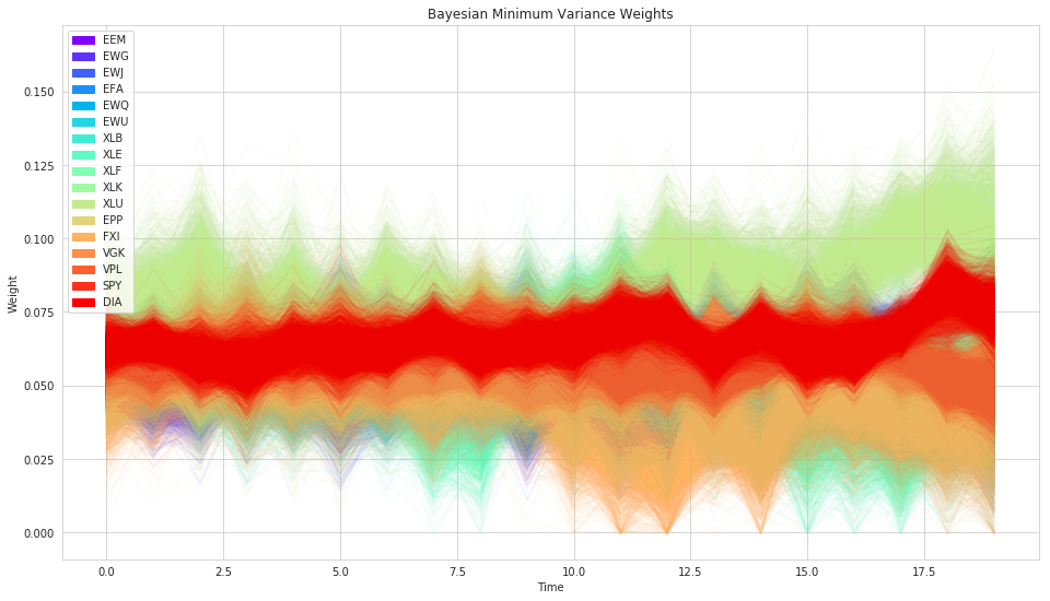
Stochastic Optimization
We have a distribution of covariances instead of single values.
So we have a distribution of possible weights.
Markowitz Weights
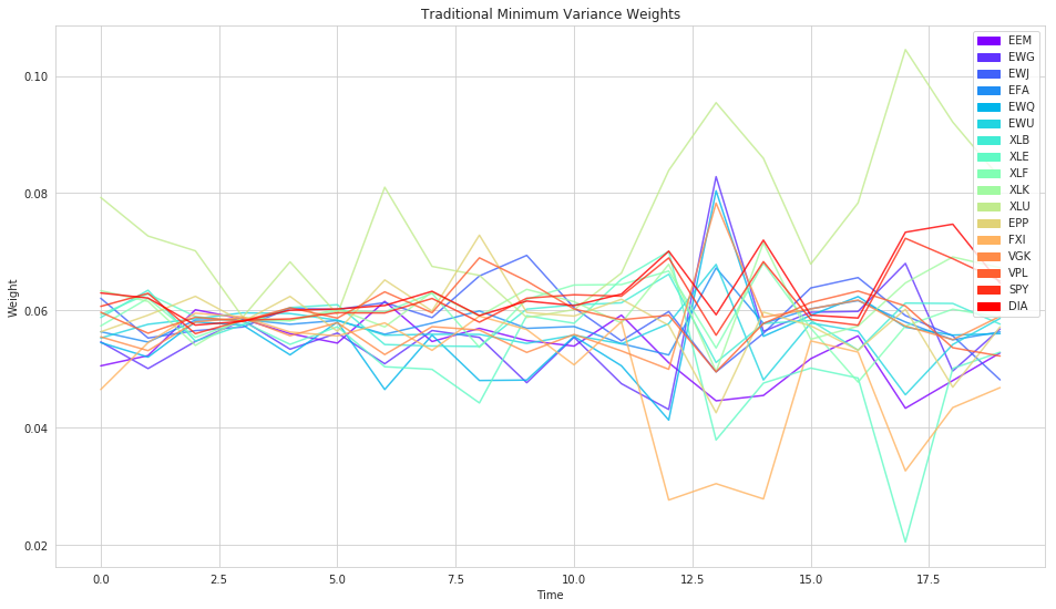
Min-Variance Portfolio
Variant of Markowitz that disregards the returns, finding the portolio with minimum variance.
Generally more stable.
Traditional Min-Variance
Bayesian Min-Variance
Evaluation
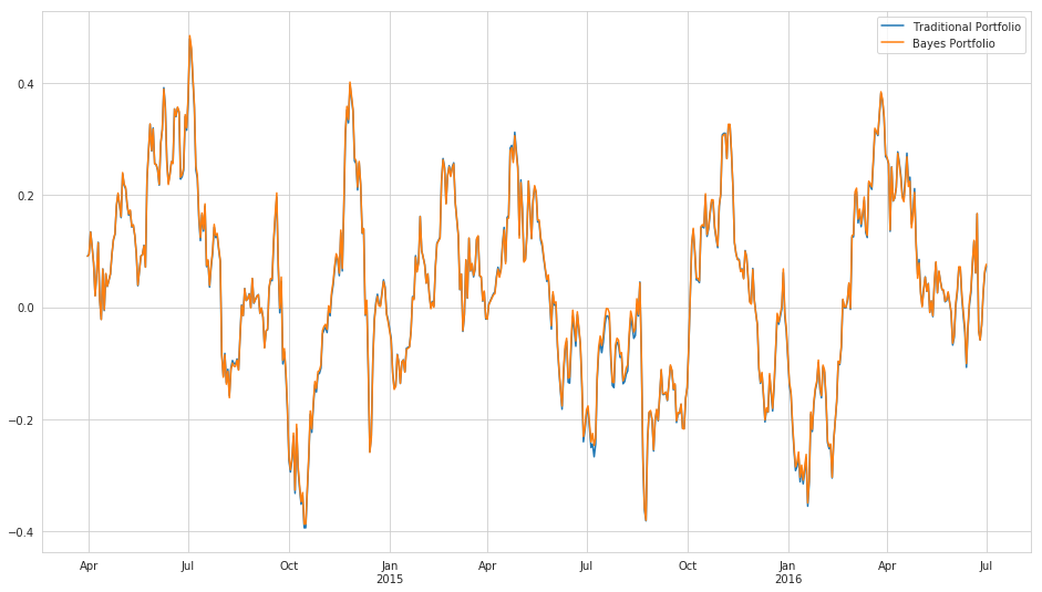
Performance
- Sharpe Ratio - $ \frac{E[R_p] - R_f}{\sigma_p} $
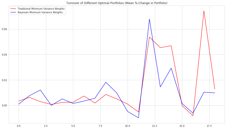
Stability (Turnover)
- Mean %-change in weights
Performance
Performance
print("Traditional Sharpe: {0}".format(trad_sharpe))
print("Bayes Sharpe: {0}".format(bayes_sharpe))
Turnover
Turnover
print('Mean Turnover:')
print('Traditional Minimum Variance Weights: ', np.mean(trad_turnover))
print('Bayesian Minimum Variance Weights: ', np.mean(posterior_turnover))
Possible Improvements
The model still leaves a few things to be desired.
Placing a random walk distribution on the Cholesky factors is weird - they don't have a straight-forward relationship to the individual elements in the covariance matrix we actually want to model.
Prediction with random walks is not very good, a Gaussian process might be better.
Maybe allow principal components of covariance matrix to change or assume a block structure to reduce dimensionality.
Compare against the Ledoit-Wolf Estimator instead of sample covariance.
- Scalability, in both number of securities and amount of time, is a major problem.
Tools
- PyMC3
- CVXPY
References
- Stochastic Volatility Model Blog Post - https://docs.pymc.io/notebooks/stochastic_volatility.html
- Q Forum Post on Hierarchical Risk Parity by Thomas Wiecki - https://www.quantopian.com/posts/hierarchical-risk-parity-comparing-various-portfolio-diversification-techniques
@clean_utensils
@mmargenot
max@quantopian.com
This presentation is for informational purposes only and does not constitute an offer to sell, a solicitation to buy, or a recommendation for any security; nor does it constitute an offer to provide investment advisory or other services by Quantopian, Inc. ("Quantopian"). Nothing contained herein constitutes investment advice or offers any opinion with respect to the suitability of any security, and any views expressed herein should not be taken as advice to buy, sell, or hold any security or as an endorsement of any security or company. In preparing the information contained herein, Quantopian, Inc. has not taken into account the investment needs, objectives, and financial circumstances of any particular investor. Any views expressed and data illustrated herein were prepared based upon information, believed to be reliable, available to Quantopian, Inc. at the time of publication. Quantopian makes no guarantees as to their accuracy or completeness. All information is subject to change and may quickly become unreliable for various reasons, including changes in market conditions or economic circumstances.